Why calibration intervals on SIS transmitters become a cost and risk problem
A typical plant sets one calibration interval for every pressure transmitter in the safety-instrumented system (SIS) at start-up. Years later, that number is still in the maintenance system, and nobody remembers where it came from. Every calibration means a bypass or override, a permit, isolation, and access to a device that may sit in a hazardous area. Each visit also exposes the technician to some risk, leaves protection reduced for a while, and carries a real chance of leaving the loop in the wrong state.
Stretching intervals blindly is no fix. Drift is one of the ways a safety transmitter fails dangerously without telling anyone. Extend the interval without evidence and the probability of failure on demand (PFD) the design assumed may quietly stop being true.
The way out is to treat the calibration interval as a hypothesis, something as-found data either confirms or knocks down. Those same data also have to square with the proof-test interval used in the SIL verification.
Standards and requirements context
Three documents frame the discussion:
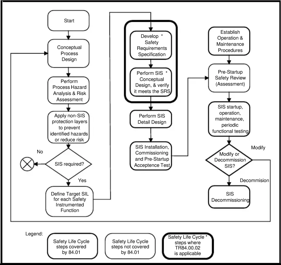
IEC 61511covers functional safety for safety instrumented systems in the process industry sector. It puts responsibility on the owner/operator to define proof-test procedures and intervals, verify that the SIS meets its required integrity, and manage changes to those assumptions. It also expects the user to justify equipment for a given application, including through documented operating experience (prior use).IEC 61508is the generic functional safety standard for electrical, electronic and programmable electronic safety-related systems. It underpins the manufacturer's FMEDA and the safety manual that comes with a certified transmitter.ISA-TR84.00.02is the technical report on SIL verification techniques. It gives the simplified equations people actually use to relate failure rates, proof-test interval and PFD.
In practice, two documents govern any change. The first is the transmitter's safety manual, which gives the dangerous undetected failure rate and the assumptions behind it. The second is the SIL verification calculation for the loop, which fixes the proof-test interval and the proof-test coverage the design relied on.
Calibration is not the same as a proof test
People mix these two up all the time, and the mix-up drives bad decisions in both directions.
- Calibration compares transmitter output with a traceable reference across the range and adjusts it if needed. It quantifies drift, which is one failure mechanism.
- Proof test is a periodic test designed to reveal dangerous undetected failures across the whole sensing function. That is more than the sensor. It covers impulse lines and manifold, process connection, output signal path, the response of the logic solver input, and ideally the final-element action.
A calibration alone rarely gives full proof-test coverage. A plugged impulse line or a closed root valve won't show up if the calibrator is connected downstream of it. On the other hand, a well-designed proof test that applies pressure through the process connection can catch both drift and blockage.
The simplified relationship for a single (1oo1) element is:
PFDavg ≈ λDU × TI / 2
where λDU is the dangerous undetected failure rate and TI is the proof-test interval. With imperfect proof-test coverage C, a common refinement is:
PFDavg ≈ C × λDU × TI / 2 + (1 − C) × λDU × LT / 2
where LT is the lifetime or the interval to a more complete test or replacement. Two consequences follow:
- If the calibration is the proof test, lengthening it raises PFDavg in direct proportion. The extension has to fit inside the margin the SIL verification already has.
- If coverage is poor, the (1 − C) term is paid over the whole lifetime. Better coverage is often worth more than a shorter interval.
Building the justification: from specification to field data
Start from the manufacturer's stability data
Neither a regulator's general recommendation nor a habit tells you how a particular transmitter in a particular service will behave. The stability specification gives you a first estimate, and so does Fuji Electric's calculation method. It sets the interval from the accuracy you need and the drift the device is specified to show over time.
Validate with your own as-found data
Specification values describe a population under reference conditions. Your service adds vibration, temperature cycling, overpressure events, process fouling and seal-fluid effects. After two to three calibration cycles, analyse the actual as-found drift for each sensor and decide whether the interval holds up.
What you analyse matters more than how many cycles you have:
- As-found error at zero and at span, recorded before any adjustment. Adjust first and you've destroyed the evidence.
- Direction and consistency. Random scatter inside the calibrator's uncertainty tells a different story from steady movement in one direction.
- Grouping. Transmitters of the same model, range, service and mounting can be pooled, but only if they behave statistically alike. A wet-gas separator and a dry fuel-gas header are different populations.
- Calibration standard uncertainty. If the reference and procedure can't resolve the drift you're trying to catch, the data can't support an extension.
Comparing interval-setting approaches
| Approach | Basis | Strength | Weakness |
|---|---|---|---|
| Fixed interval for all devices | Legacy practice or a site rule | Simple to schedule | No link to SIL assumptions or actual behaviour |
| Specification-based calculation | Manufacturer's stability and required accuracy | Defensible starting point, quick | Ignores service conditions |
| Data-driven, per device or group | As-found history and trend | Reflects real drift; supports extension or shortening | Needs disciplined records and a defined tolerance |
| Data-driven plus online comparison | As above, plus deviation monitoring between redundant transmitters or against a related measurement | Detects drift between tests | Credit in PFD only if validated and documented |
Illustrative worked example: drift rate from a stated specification
The specification values below come from the Fuji Electric method. The scenario around them is illustrative, not a real plant case.
Stated: a transmitter with an upper range limit (URL) of 320 mbar, and a stated maximum drift of ±0.32 mbar over 10 years.
- Drift as a fraction of URL: 0.32 mbar ÷ 320 mbar = 0.001, which is 0.1 % of URL over 10 years.
- Annual drift rate: 0.32 mbar ÷ 10 years = 0.032 mbar per year.
- Monthly drift rate: 0.032 mbar/year ÷ 12 months/year = 0.00267 mbar per month.
This assumes drift accumulates linearly, which is a simplification. The 0.032 mbar per year figure is a specification envelope, not a prediction for your device.
Illustrative reading of the result. The annual figure is very small. Before field data can justify an extension, the calibration reference and procedure must resolve differences of this size. If the calibrator's uncertainty and the reading resolution are larger than the drift you'd expect between two visits, the as-found results will show mostly noise. In that case the data can't support a longer interval, and they can't prove drift is absent either.
Decision logic. Suppose the as-found record, across the initial 12-month interval and the following two to three cycles, stays inside the loop's defined tolerance. Suppose there's no consistent direction, and the reference was good enough to see real movement. That supports a stepwise extension. If any as-found result lies outside tolerance, or a trend is heading toward it, hold or shorten the interval and investigate. The tolerance itself has to come from the loop's safety requirements and the SIL verification, not from the manufacturer's accuracy statement.
Keeping SIL integrity intact when you extend
- Re-run the SIL verification with the new interval. Use the safety manual's λDU and the proof-test coverage you can actually demonstrate. If PFDavg no longer meets the target, the extension is not permitted, whatever the drift data say.
- Extend in steps. Take one step, collect another cycle of as-found data, then decide on the next.
- Treat out-of-tolerance as-found results as potential dangerous failures. Record them, find the cause, and feed them into the failure-rate assumption. A pattern across a group of devices challenges the prior-use argument.
- Separate calibration from the proof test where that helps. A full proof test through the process connection can stay on its own interval while a lighter calibration check is adjusted. Check that the coverage claims still hold after the split.
- Credit online diagnostics carefully. Deviation alarms between redundant transmitters can catch drift between tests. Credit them only where the detection is validated, alarmed, and acted on within the process safety time.
- Manage the change formally. The extension changes the safety lifecycle documentation. Update the proof-test procedure, maintenance system and verification report together.
Safety precautions for field calibration and proof testing
Any work that isolates, vents or connects to a transmitter on hydrocarbon service needs these controls:
- Get an approved SIS bypass or override with documented compensating measures, and confirm the process condition allows it.
- Isolate the transmitter at the root or block valves per the permit, and lock out (LOTO) the isolation points.
- Depressurise through the vent or bleed route to a safe location, such as a closed drain or flare, never to the work area.
- Verify zero energy at the transmitter before disconnecting any fitting.
- Run gas detection during venting and while the impulse line is open, and apply hazardous-area precautions. Use certified calibrators and tools suitable for the zone.
- After the test, restore the process connection, leak-test it, confirm the output reads correctly against the process, and remove the bypass with a documented check.
Checklist: before you extend an interval
- Identify the transmitter model, range and service, and confirm the current interval and what the SIL verification assumed.
- Confirm whether the calibration is part of the proof test, and what coverage it gives for impulse lines and the process connection.
- Collect as-found data from every cycle, recorded before adjustment.
- Check that the calibration reference and procedure can resolve the drift expected between visits.
- Define the as-found tolerance from the loop's safety requirement, not from the datasheet accuracy.
- Look at trends and drift direction, not just pass/fail results.
- Pool devices only where model, range and service are alike.
- Re-run the PFDavg calculation with the proposed interval and confirm it meets the target.
- Review any out-of-tolerance event and its effect on the failure-rate assumption.
- Approve through management of change, and update the procedures and maintenance schedule.
- Re-evaluate after the first extended cycle.
Conclusion and next steps
Start with the transmitters that have the longest clean as-found history and the most consistent service conditions. Confirm your reference equipment can resolve the drift you expect, and re-run the PFD calculation before touching the schedule. Where the evidence is thin, keep the existing interval and improve the data first. For the worked basis, read Emerson's technical note and Fuji Electric's calculation method alongside the transmitter safety manual.